Viscoelasticity
The vast majority of fluids studied using rheology are viscoelastic and almost all processes are non-linear, that is, they involve significant deformations. This is indicated by the large upper section in the Pipkin diagram in Figure 2. A viscoelastic fluid converts part of the deformation energy into heat (viscous deformation) and stores part of the energy (elastic deformation). Viscosity thus not only describes a part of viscoelasticity but also requires us to measure it so that the elasticity does not affect the measurement. To describe viscoelasticity, moduli are typically used.
Unfortunately, models and methods for measuring linear viscoelasticity are easily available. Although much research is taking place on non-linear models and methods, so far there are no simple models that have a clear link to real world parameters and the structure of fluids. See, for example, [6] for an overview of non-linear viscoelasticity.
Linear viscoelasticity means that the fluid does not deform so much as to break down the structural elements, which in practice means that it is only possible to deform a millimetre-sized samples no more than a few micrometres. To be able to apply the linear viscoelasticity model, we must first examine how much deformation the fluid can take. Even though the maximum deformation is much smaller than in the processes we are interested in, methods for linear viscoelasticity are frequently used. These are called small amplitude oscillatory shear (SAOS) tests and are valuable because they nicely describe transitions, such as melting, gel formation and crystal formation, and because the results can be related to the structure of the fluid.
Characterisation of linear viscoelasticity is usually done as in Figure 7. The fluid is applied in a measuring system, for example between two concentric cylinders as in the figure. The cup is oscillated at a constant frequency, and the fluid transmits energy to the inner cylinder. The added deformation and the resulting torque are recorded, and the complex shear modulus is calculated from the deformation and torque as well as the phase shift, or phase angle, between the two sinusoidal signals. If the fluid is completely elastic, the signals are in phase and the phase angle is δ=0. If the fluid is a Newtonian liquid, the signals are out of phase and the phase angle is δ=90°.
The complex shear modulus G* consists of two components, one viscous and one elastic. This provides an analogy to complex mathematics, which facilitates the description of G* as consisting of a real part, the storage modulus G′, and an imaginary part, the loss modulus G″. This can be expressed as
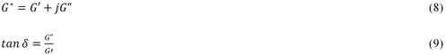
where j2 = -1.
Without delving into the details of the mathematical background, we can conclude that two parameters are needed to describe the complex shear modulus and that we can choose arbitrarily between | G*|, G′, G″ and δ. For example, we can choose the pair storage modulus G′ and phase angle δ, and think of the modulus G’ as a rigidity, albeit only for very small deformations, and the phase angle δ as a description of the nature of the fluid between δ=0 for a solid and δ=90° for a liquid. But, as stated, it is up to the individual to choose any two of the parameters.
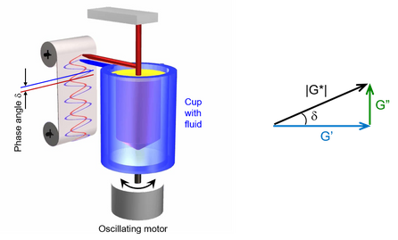
Figure 7. The principle for determination of the complex shear modulus.
Important concepts
The complex shear modulus G* describes both elastic and viscous behaviour for a fluid. G* can be divided into the storage module G′ and the loss module G. Their relationship is expressed using the phase angle δ as tan δ=G″/G′.
Mechanical spectrum
To better understand the importance of the complex shear modulus, we can take bouncing putty or silly putty – as an example. Many people have had this bouncing putty as a toy. If you haven’t, why not buy a jar, or at least search bouncing putty on YouTube. As its name suggests, bouncing putty behaves both as a malleable clay and as a bouncing ball; see the images in Figure 8. If we vary the frequency in an experiment, we get a response that goes from typical liquid-like behaviour to the behaviour of an elastic material. At low frequencies, the storage modulus for the bouncing putty is greater than the loss modulus and the phase angle close to 90°. At high frequencies, the inverse applies and the phase angle is close to 0°. We can think of frequency as a measure of how quickly we deform the fluid. Low frequencies mean slow changes that reflect the behaviour as the bouncing putty flows out. When you bounce it, the deformation is rapid and corresponds to a high frequency.
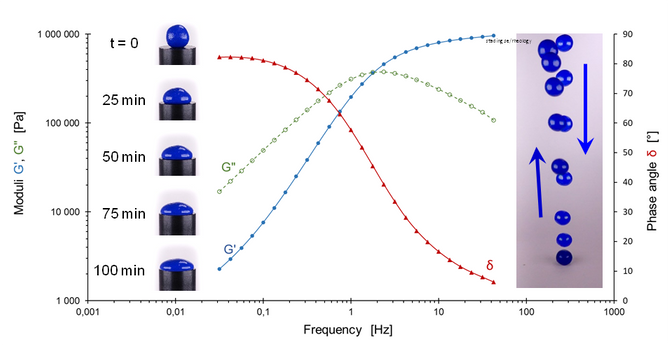
Figure 8. Mechanical spectrum for bouncing putty. The left photos show a ball of silly putty slowly flowing out during 100 minutes and the right overlaid photos show the same ball bouncing with 40 ms in between each photo.
The bouncing putty’s behaviour is typically viscoelastic and fits well into the middle section of Figure 2. The bouncing putty has a relaxation time of 2 s, and time corresponds to one period of the oscillation, which is our observation time. Thus, at a frequency of 2 Hz, the Deborah number is 1. If we increase the frequency, we reduce the observation time and therefore move to the right in Figure 2, towards the behaviour of elastic materials, and the corresponding for decreasing frequency when we move to the left.
Important concepts
Extensional viscosity is always at least three times shear viscosity. The extensional viscosity reflects the elasticity of the fluid, and when the fluid is elastic the Trouton ratio is greater than 3.
Slow motion of bouncing putty, click to start video.
Time-lapse video of flowing bouncing putty, click to start.
Viscoelasticity and transitions
The great advantage of SAOS is that we can follow transitions in fluids. Figure 9 shows how egg white forms a gel with rising temperatures, which is what happens when we boil an egg. At room temperature, the egg white is liquid and even if δ is not 90°. As the temperature increases, G′ increases faster than G″ and when the albumin in the egg white coagulates and forms a three-dimensional network, then G′ becomes much greater than G″. This can be followed thanks to the fact that the measurement technique is linearly viscoelastic, that is, the deformation is so small that the fluid springs back without breaking any structure. Figure 9 shows that the egg white solidifies just above 75°C when the storage modulus G′ rises sharply. However, the phase angle shows that the egg white already at a low temperature has a structure (δ<40°) and that gel formation is also underway below 75°C because the phase angle is continuously decreasing.
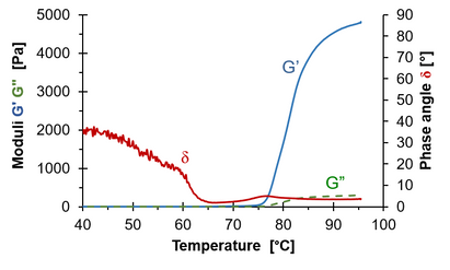
Figure 9. Storage modulus G′, loss modulus G″ and phase angle δ for egg white as a function of increasing temperature.
Relationship between linear viscoelasticity and viscosity
It is possible to define a complex shear viscosity η* using the unit Pa·s, similar to the shear viscosity we discussed earlier
where ω=2πf and f is the oscillation frequency. Thus, |η*|=G*/2πf.
Empirically, we know that the complex viscosity is often equal to the shear viscosity we previously defined, i.e.
This empirical rule is called the Cox-Merz rule and applies to fluids without structures broken down by the shear deformation [7]. For example, the rule works for Newtonian oil and non-Newtonian beverages and soups, but not for pudding-like materials like yoghurt.
Important concepts
The Cox-Merz rule provides an empirical relationship between shear viscosity and linear viscoelasticity.
Measurement methods for quality control, processing and kitchens
Rheometers are expensive, and everyone who needs to characterise a fluid does not have access to a measuring instrument. This means that simple measurement methods abound. It is especially true in industry, where quality control is necessary. There are countless different texturometers that are well established in their respective areas and described in different guidelines and standards [8]. The methods often use simple geometries, such as flow out of a hole in a cup or syringe, flow in a channel, penetrating probes and sagging of semi-solids.
Flow in a channel or radially on a surface is used for tomato paste (Bostwick consistometer) and cheese (Schreiber test), for example, and corresponding methods are used on a larger scale for cement and concrete. The Bostwick method, which provides a measure of the ratio of density to shear viscosity, has also been used to measure the thickening rate of texture-modified beverages for dysphagia treatment.
Similarly, the International Dysphagia Diet Standardisation Initiative (IDDSI) scale uses the time it takes for a fluid to flow out of a syringe as a measure of the degree of the fluid consistency. Similarly, back extrusion is also used as a measure of consistency. This is the force required to push a piston into a cylinder, where the fluid can penetrate up along the perimeter. Both of these methods involve complex flows and are difficult to interpret scientifically.
Some methods are both simple and well-characterised in the scientific literature, such as the slump test for determining yield stress for cement dispersions. In this test, cement is poured into a container, the container is lifted and a measure is then taken of how much the contents collapse, or slump [9]. This gives a surprisingly accurate measure of yield stress. The corresponding method for gelatine, the Bloom test, involves compressing a cylindrical gel, and the force needed to compress it four millimetre is the Bloom value. This can be related to the molecular weight of gelatine, but it is not as well studied scientifically as the slump test.
There are both advantages and disadvantages to these simple methods.
Advantages
- Performed quickly.
- Do not require expensive equipment.
- It’s better to measure something than nothing at all.
Disadvantages
- They measure only at one strain rate (see how different results can be obtained for syrup compared with xanthan in Figure 4).
- Often complex flow, with both shear and extensional flow.
- Difficult to relate to pure viscosity or viscoelasticity.
Another approach is to use process equipment, such as mixers, to measure shear viscosity. This is called systemic rheology, and its theory was developed in France [10]. Traditional viscometric methods use measurement systems with well-defined geometry that provide as simple and homogeneous a shear field as possible; compare with Figure 3. In a mixer, the geometry is designed to create maximum stirring rather than a homogeneous shear field, but the energy consumed during the stirring is still a measure of fluid viscosity. The systemic rheology method uses a calibration procedure with two calibration fluids, one Newtonian and one non-Newtonian. A Newtonian oil and a shear-thinning polymer solution are usually used.
It might seem like a joke, but systemic rheology provides surprisingly accurate viscosity measurements using simple means, even for an ordinary electric mixer; see Figure 10. A power meter was connected to an electric hand mixer that was calibrated with two fluids that were first characterised with a scientific grade viscometer. Figure 10 shows the results of measuring a jam. The measurements cover a small shear rate range depending on the fixed speeds of the electric mixer, but the measured viscosity is quite accurate compared with the viscometer. They also show that the jam is shear-thinning, which a one-point measurements otherwise would not show.
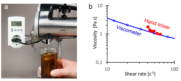
Figure 10. Determination of the viscosity of a jam by a calibrated hand mixer and an electric power meter.
Important concepts
Systemic rheology is a method of measuring viscosity using irregular geometries, such as mixers.
Rheology literature
There are many textbooks in rheology at different levels covering different sub-areas. I want to mention three text books suitable for further reading.
- Barnes, H. A., Hutton, J. F., & Walters, K. (1989). An Introduction to Rheology Elsevier Science Publishers, ISBN 9780444871404
The book covers most areas of rheology and it covers rheology in depth contradictory to the title. - Mezger, T. G. (2006). The Rheology Handbook: Vincentz Network, doi:10.1515/9783748600367
The book is experimental in nature and covers all areas of rheology. - Macosko, C. W. (1994). Rheology Principles, measurements and applications. New York: VCH Publishers, ISBN 978-0-471-18575-8
Based in fluid dynamics this book provides substantial insight in theory and application of rheology. It is also more mathematically challenging than the two books above.
References
- Pipkin, A.C., Lectures on Viscoelasticity Theory. 1972: Springer, New York.
- Macosko, C.W., Rheology Principles, measurements and applications. 1994, New York: VCH Publishers.
- Barnes, H.A., J.F. Hutton, and K. Walters, An Introduction to Rheology 1989: Elsevier Science Publishers.
- Barnes, H.A. and K. Walters, The yield stress myth. Rheol. Acta, 1985. 24: p. 323-326.
- Nystrom, M., et al., Effects of rheological factors on perceived ease of swallowing. Applied Rheology, 2015. 25(6): p. 40-48.
- Hyun, K., et al., A review of nonlinear oscillatory shear tests: Analysis and application of large amplitude oscillatory shear (LAOS). Progress in Polymer Science, 2011. 36(12): p. 1697-1753.
- Cox, W.P. and E.H. Merz, Correlation of dynamic and steady flow viscosities. Journal of Polymer Science, 1958. 28(118): p. 619-622.
- Mezger, T.G., The Rheology Handbook. 2006: Vincentz Network.
- Pashias, N., et al., A fifty cent rheometer for yield stress measurement. J. Rheol., 1996. 40(6): p. 1179-1189.
- Aït-Kadi, A., et al., Quantitative Analysis of Mixer‐Type Rheometers using the Couette Analogy. The Canadian Journal of Chemical Engineering, 2002. 80: p. 1166-1174.