INTRODUCTION TO RHEOLOGY
FOR EDUCATED BEGINNERS
The ketchup will not come out of the bottle, the concrete does not fill the mould or the paint drips. These are all problems which can be explained and solved by rheology. This science is defined as the study of the flow of matter and deals with liquids and semi-solid fluids. Rheology covers all types of fluids ranging from food and plastics to mud and glaciers. The common denominator is that the fluids behave intermediate in between water and a solid.
Even a solid material flows, that is, if we are patient enough to wait it out, which Heraclitus pointed out already 500 BC – panta rei, everything flows. In practice we do not need to consider the flow of for example a construction material as the relevant flow time usually is longer than the lifetime of the material. And using fluid dynamics for describing the flow of water we instead assume instant flow. By using rheology we know when we need to consider the flow or not, and rheology will guide us to the correct model to describe a specific flow or fluid.
This text describes different rheological models – when they are applicable and which results they may give. Many of the examples are taken from the food area as the rheological behaviour of foods is known by all of us. The level is adjusted to educated beginners, that is someone with some background in science but with no prior knowledge of rheology.
Substances that flow are sometime referred to as a material and sometimes as a liquid. It will here be referred to simply as fluid. This means that a fluid can be thin as water or thick as pudding, yet be referred to as a fluid.
Important concepts
A fluid is a substance that continuously deforms under external forces. The term will here be used for all substances, for materials, semi-solids, liquids and similar.
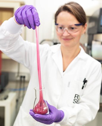
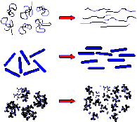
Figure 1. Rheologist Johanna Andersson demonstrates the viscoelasticity of slime
Thin or viscous – different rheological models
Most people have heard of the term viscosity and know that a viscous substance exhibits high viscosity. Viscosity is an adequate word for describing the state of an egg white when we crack an egg, for example. But when an egg is boiled and it solidifies, viscosity becomes irrelevant for describing the consistency of the boiled egg. In that case, it is more relevant to describe how elastic the boiled egg is when we bite into it. So, different models are needed for different situations.
Allen Pipkin’s overview of different rheological models is often used to determine the right model for a specific fluid and situation; see Figure 2 [1] The x-axis displays the Deborah number, which is the ratio between the time it takes for a fluid to relax or flow and how long we observe the flow. So, we find water at the left and pudding at the right of the diagram. The y-axis displays the degree of deformation – how much we deform the fluid.
At the far left of the diagram are fluids that have a constant viscosity. These are called Newtonian fluids. The Newtonian model works when we have a fluid that relaxes quickly in relation to observation time, like water and other beverages. In our ordinary physical world, however, we rarely perceive things that happen faster than tenths of a second, and the Deborah number is therefore low when we apply it to beverages. On the far right of the diagram, we see the opposite phenomenon. Here, we have fluids that would be perceived as extremely viscous or, even more likely, as solid materials. These are called elastic materials. Examples of elastic foods are flaky biscuits and hard cheese. All construction materials also fall under elastic materials.
To understand high Deborah numbers, let’s image a bookshelf that we load with heavy books. The bookshelf will give way under the weight of the books, but will spring back when we remove them. However, if we think of a cheap bookshelf that we loaded with heavy books ten years ago, we can sometimes note a residual deformation when we remove the books. The shelf curves downwards even after we remove the books. This shows that the long observation time of ten years is longer than the relaxation time of the shelf material. In the Pipkin diagram, this means that the Deborah number is indeed high, but does not extend into the area for elastic materials.
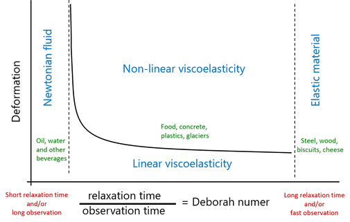
Figure 2. Overview of different models describing material properties of viscous fluids. Freely reproduced from [1] and [2].
In reality many fluids end up in the middle area, especially food and other biological fluids. Because these fluids are both viscous and elastic, they are called viscoelastic. Many processes, such as pumping, eating, swallowing and stirring, involve deforming and reshaping the fluid, so the predominant area in Figure 2 is non-linear viscoelasticity. This is where most fluids lie. Unfortunately there are few simple and well-defined measurement methods for non-linear viscoelasticity, although much research is taking place. On the other hand, well-established methods are available for measuring linear viscoelasticity, called small amplitude oscillatory shear (SAOS) tests, since linear viscoelastic fluids do not deform more than that they can linearly return to their original state. Even though few processes are linear, the methods are important for enabling us to study melting, gel formation and other transitions.
It is now time to review what material properties we can measure for different fluids under different conditions. But first, we need a suitable way to express forces and deformation.
Stress and strain
A flow is caused by forces and causes fluids to deform. A large surface produces greater resistance than a small one, and in order to ignore geometry we can measure the resistance as a stress rather than a force and express it as force per unit area. And instead of absolute deformation we can use a dimensionless deformation called strain. The strain caused by a force acting parallel to a surface is known as shear strain, and the strain caused when a material is subject to tension due to elongation is called tensile strain. Since viscosity depends on how fast a flow is, we also need to express the speed of the strain as shear rate in shear and extension rate in extension.
A normal flow causes the fluid to deform in shear mode. To understand this term, we can first study simple shear in Figure 3a. Shearing means that a force F acts along a plane, while under elongation it acts perpendicular to a plane (Figure 3d). The fluid velocity is zero at the lower stationary plane and v at the upper plane in Figure 3a. Because the velocity is constant, deformation increases linearly from the lower to the upper plane and the shear rate becomes
Similarly, in the pipe flow in Figure 3b we see that the velocity is greatest in the centre of the pipe and that it decreases to zero at the pipe wall. If we divide the flow into thin layers and straighten the layers, we can understand the analogy of simple shear in Figure 3a. In the pipe flow, however, the velocity varies quadratically over the cross section of the pipe. The shear strain is the derivative of the velocity (equation 1) and therefore varies linearly, from zero in the centre of the pipe to the maximum value at the pipe wall.
Figure 3c shows the flow through a contraction in the pipe. The fluid is forced to extend in the direction of the flow in order to pass through the contraction. This gives rise to a strain, and we can similarly calculate a tensile stress, still as a force per unit are, and a strain rate as dvz/dz. Since the flow rate also varies with the pipe diameter, the fluid is exposed to shearing at the same time.
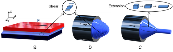
Figure 3. Different categories of deformation in flow. a) Simple shear. b) Shear in pipe flow. c) Extension in contraction flow. The blue fluid shows the flow inside the pipes in b) and c).
Shear viscosity
Viscosity expresses resistance to flow and is a relevant parameter for the left part of the Pipkin diagram (Figure 2). A viscous fluid thus has a higher viscosity than a more liquid fluid, such as syrup compared with water. In most cases, we are trying to deform the fluid in shear (Figure 3a-b), like the flow in a pipe, but a fluid has an even greater resistance to stretching (Figure 3c). The extension occurs when we try to squeeze the fluid through a contraction, like when we swallow or force a fluid out of a nozzle. The viscosity is always at least three times greater in extension than in shear mode. There is therefore both a shear viscosity and an extensional viscosity, which however are not equal.
Now, we can first define the shear viscosity η
where η is expressed in units of Pascal-seconds, Pa·s=Ns/m2, σ is the shear stress in units of Pa=N/m2 and is the shear rate expressed in units of s-1. Both the shear viscosity and the extensional viscosity depend on how quickly we deform the fluid rather than on how much we deform it. Shear viscosity is used much more frequently than extensional viscosity, and in everyday language viscosity is usually synonymous with shear viscosity. The same applies in this text, and shear or tension will only be indicated when relevant to the context.
The shear rate varies depending on the process. In slow flows like sedimentation the shear rate is low, typically ≤10-4 s-1. But it is high in processes involving flow in thin layers, such as when we apply skin cream or coat paper, typically ≥104. However, many processes including chewing, swallowing, stirring and pipe flows fall somewhere between these extremes, usually 0.1–1000 s-1. See Figure 4 for common shear rate ranges.
Viscosity also varies greatly – from water (10-3 Pa·s at 20°C) to molten plastic (103 Pa·s) and asphalt (108 Pa·s), see Figure 4 [3]. All these levels are approximate because we will later see that viscosity depends on several different parameters. Equation 2 describes the simplest model for a fluid, a Newtonian fluid for which the viscosity is constant and independent of shear rate. As mentioned earlier, this applies for oils but is otherwise unusual for food and beverages. The viscosity usually depends on the shear rate, as well as temperature and other parameters. The main parameters influencing viscosity are presented here individually.
Viscosity and shear rate dependence
The vast majority of fluids we come across, such as food, skin creams and paint, have a viscosity that decreases with increasing shear rate. This means that they are perceived as more thinner the faster we stir them. This behaviour is called shear thinning or pseudoplasticity and is illustrated in Figure 4. Xanthan, which is a strongly shear-thinning thickener (E415), consists of long polysaccharide chains. In rapid flow, they line up in the flow and take up little space, thus exhibiting little resistance. In slow flow, however, they take up more space and exhibit greater resistance. Other polymers like hyaluronic acid used in medical applications behave in the same way, making it possible to apply them with a syringe or microneedle.
The inverse behaviour, shear-thickening or dilatant, is unusual but spectacular. You can find one of the few practical examples mixing equal parts of cornflour and water, which you can even walk on thanks to its high resistance at high shear rates (see example on Youtube). But food is thankfully not shear-thickening, it would present immediate danger when swallowing.
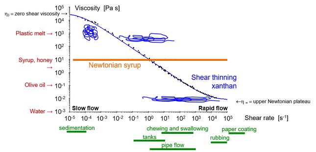
Figure 4. Shear thinning of a solution of xanthan compared to a Newtonian syrup. Green text gives typical shear rate ranges for common flows and red text the viscosity for some common fluids.
Important concepts
A fluid with constant viscosity is called Newtonian. If the viscosity decreases with increasing shear rate (faster flow or faster stirring), the fluid is shear-thinning or pseudoplastic. The inverse, when the viscosity increases with increasing shear rate, is called shear-thickening or dilatant.
Different mechanisms causing shear thinning.
Viscosity and time dependence
Viscosity depends on fluid structure, like the polysaccharide chains in our xanthan example. If we stretch molecular chains by flow, the chains immediately contract as the flow slows down, while in other cases the structure breaks down as we deform it. Yoghurt is a typical example. When we open a package of set-type yoghurt, the consistency is pudding-like but becomes more fluid when we stir it. The stirring adds mechanical energy that breaks down the protein structure. If we let the yoghurt rest, the structure rebuilds and the viscosity returns to its original value. This behaviour is called thixotropy. Similar behaviour is also found in household paints, and the technical advantage here is that pigment particles are prevented from settling during storage and transport. The reconstituting of the structure is usually a slow process that takes hours.
Thixotropy is common in food, although structural regeneration is not always 100 percent. It is common for structures in fluids that we eat, but it is not as common for them to completely return to their original structure. The inverse phenomenon of thixotropy also exists when the added mechanical energy creates structure. It is called rheopexy and is unusual.
When characterising the shear rate dependence of fluids, as in Figure 4, it is impossible to determine whether the behaviour is due to thixotropy or shear thinning. When we determine the viscosity curve, we make stepwise increases in shear rate with a sequence of point-wise measurements, which takes time. So it may very well be as likely that the structure is broken down by the mechanical energy as the fluid is shear-thinning. To address this issue, we usually do double shear rate sweeps, that is, with an increasing and a decreasing sequence of shear rates. Figure 5 shows four sequences for a cheese sauce, and we can conclude that it is both thixotropic and shear-thinning. To be precise, Figure 6 shows that the cheese sauce is shear-thinning and that its structure is broken down by the shear strain. To conclude it to exhibit true thixotropy would require a rest period with repeated shearing.
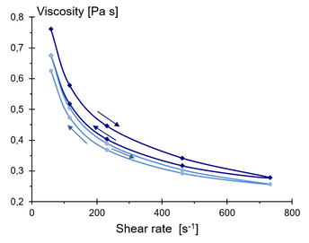
Figure 5. Viscosity as a function of shear rate for a cheese sauce showing that the sauce is shear thinning and that the structure breaks down during prolonged shearing.
Temperature and pressure effects on viscosity
Viscosity decreases with increasing temperature. It is due to individual elements or particles in the fluid attracting each other across flow lines. As the temperature increases, the increased thermal energy causes an increase in molecular mobility and counteracts the attraction. Temperature dependence can often be described using a simple Arrhenius-type equation
where η denotes the shear viscosity and T temperature. A and B are constants.
Temperature dependence has many implications. If we want to measure exact viscosity, it is crucial to keep the temperature constant. For ±1 percent accuracy in the viscosity value, we typically need to keep the temperature within ±0.3°C. The temperature effect is something we observe in everyday life. We heat the bottle of syrup in the microwave oven to more easily get it out and we melt plastics to shape them. The temperature effect is also noticed when eating as the viscosity of a fluid food such as a soup heated from 20°C to 37°C typically is halved.
Viscosity increases with increasing pressure, but extreme pressure is needed before we can observe it. The effect of pressure is important in processes like off-shore oil drilling far below the seabed (~200 times atmospheric pressure) and in lubrication of internal combustion engines (~10,000 times atmospheric pressure). But for medical applications and food, the pressure effect is negligible.
Important concepts
Thixotropy describes how the structure of a fluid breaks down during deformation, and then builds back up when deformation ceases. The unusual and inverse phenomenon, structure building at deformation, is called rheopexy.
Viscosity decreases with increasing temperature.
Viscosity increases with increasing pressure, but it is only relevant for extreme pressures.
Viscosity and yield stress
Dependence on a yield stress can most easily be described as the ketchup effect, meaning that the fluid does not flow until you exceed a threshold – the yield stress. For ketchup, this happens when we shake the bottle, and once the ketchup starts to move it can be described by its viscosity. But before the yield stress is exceeded, the fluid behaves like a solid material. Since Heraclitus already established that everything flows provided we wait, yield stress may seem like a paradox, in other words, yield stress is only an effect of our observing the flow for too short a time. This has given rise to many academic discussions [4] but has resulted in a compromise that, like the Pipkin diagram, takes into account observation time. We do not want to wait for hours on end to put ketchup on our food, and if we want to start a process we make sure that the pump exceeds the yield stress within a reasonable time. Yield stress does exist if we relate it to the timescale of the process. But it is also important to realise that yield stress thus depends on how quickly we measure it – it will be lower the longer we allow it to be measured.
Ketchup has a yield stress of about 15 Pa, and there are more examples of yield stress in food, from mayonnaise at 100 Pa to peanut butter at 2000 Pa. Another everyday example is toothpaste, which has such a high yield stress that it kindly remains on our toothbrushes after we squeeze it out of the tube.
Yieldstress in toothpaste, click to start the video.
Models for shear viscosity
There are a plethora of models that describe how shear stress is due mainly to shear rate and yield stress. We have already come across the simplest model in equation 2, where the shear stress is proportional to the shear rate by a constant, that is, the viscosity η. The models are usually named after their authors and the most common can be described, with increasing complexity, as
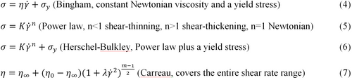
where 𝜎=shear stress, Ý=shear rate, 𝜎y=yield stress, η0=zero shear viscosity, η∞=upper plateau viscosity, and constants: n=flow index or power-law index, K=consistency index, and λ and m are constants. See also Figure 6.
There are many more models used for specific fluids or, according to tradition, in specific areas. However, the Power law model is often sufficient, since many applications and processes rely mainly on medium-high shear rates (~0,1–1 000 s-1) and describe flows where any yield stress is exceeded. Models with more parameters are required for more complex flows as well as for low or high shear rates where the viscosity levels off in the respective Newton plateau; compare Figure 4. Also note that n ≠ m in the power law and Carreau models.
The behaviour of the fluid affects the velocity profile when the fluid flows in pipes. Figure 6c shows the velocity profile of a few types of fluids. The parabolic profile flattens as the fluid becomes more shear thinning, and a similar behaviour is obtained when the fluid has a yield stress. This is usually called plug flow and means that a large portion of the fluid flows at about the same velocity and is sheared only along the pipe wall. In practical contexts, this is often positive. When food undergoes heat treatment, most of the fluid stays in the pipe for the same amount of time and becomes neither underheated (microbiological risks) nor overheated (deteriorating quality).
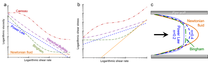
Figure 6. a) Viscosity curves and b) shear rate curves (flow curves) for the described models. c) Velocity profiles in pipe flow for the same models.
Important concepts
Fluids with a yield stress flow only when the yield stress is exceeded.
The most commonly used model for how viscosity depends on the shear rate is called Power law.
Extensional viscosity
Like shear viscosity, extensional viscosity is the ratio of tensile stress to extension rate, but the conditions are different. Extensional viscosity therefore warrants its own description.
The extensional viscosity is always at least three times greater than the shear viscosity of regular flows. For Newtonian fluids and for extremely slow flows, the ratio is exactly 3, while it can be significantly greater for elastic fluids. This ratio is called the Trouton ratio. It is especially relevant to take extensional viscosity into account when the fluid is elastic, as well as when the geometry of the flow is changed. A change in geometry can be a transition from one pipe dimension to another, flow through a nozzle, or the transition from mouth to throat during swallowing. An elastic fluid is a fluid that can store parts of the deformation energy like a coiled spring. If we want to imagine a more everyday fluid, toy slime (Figure 1) is close at hand, and for food some types of fermented milk products like ropy yoghurt. Because the energy can be stored, the flow depends on what the fluid has been exposed to earlier. It has a flow memory, and therefore behaves differently from a non-elastic fluid for which the deformation energy is completely converted into heat.
Unlike shear flow, there is a maximum for extensional flow because the fluid eventually breaks. This limit depends on the properties of the fluid and is not fully investigated scientifically. Extension is limited in many flows, as shown by the flow through the contraction in our example in Figure 3c. Like shear viscosity, extensional viscosity can vary with the extension rate and be extension-thinning or extension-thickening, even if these expressions are not as common and also not as accepted as for shear flows. In fact, a fluid may well be shear-thinning and extension-thickening at the same time. These behaviours are not connected, and even if we know that a fluid is shear-thinning we cannot predict whether it is extension-thinning or extension-thickening.
The extensional viscosity increases with the extension itself and does not reach a plateau or steady-state in the same way as the shear rate. It is not fully understood whether there is a theoretical plateau for high extensions or if the extensional viscosity passes a peak before the fluid breaks. Here, high extension mean that the fluid is typically stretched more than a thousand times its original length. This is of less interest for practical processes in which the extension is significantly lower. In practical applications, the effects of fluid elasticity are more interesting. A small elasticity acts cohesively, which is useful during firefighting when spraying water for a long period or in fountains, or for preventing droplets from bouncing off leaves when crop dusting fields. For swallowing, it has also been found that elasticity promotes safe swallowing [5]. The reason is believed to be the same as for the other applications mentioned, that is, that elasticity contributes to fluid cohesivity and sticking together during swallowing thus preventing it from entering into the airways.
Important concepts
Extensional viscosity is always at least three times shear viscosity. The extensional viscosity reflects the elasticity of the fluid, and when the fluid is elastic the Trouton ratio is greater than 3.